Multifractal analysis of heart rate data
This tutorial demo will show how to perform multifractal analysis on a database of heart rate data.
It will illustrate the use of class MF_BS_tool_inter_db to analyze an entire database in a single command.
Roberto Leonarduzzi, Patrice Abry June 2018
Contents
Setup path
Add root folder of toolbox to path (subfolders will be added automatically)
addpath ~/Documents/code/mf_bs_tool
Input data
We start by reading the data.
The file 'data_hrv.mat' contains a a part of the "Normal Sinus Rhythm RR Interval Database', made available by Phyisionet: https://physionet.org/physiobank/database/nsr2db/
The file only contains the first 6 hours of each record, in a cell array containing the time of each beat and the RR interval.
% Load the cell array data
load ('data_hrv.mat', 'data')

% Plot an example
select = 3;
figure (99)
time = data{select, 1} / 3600; % Convert time to hours
rr = data{select, 2};
plot (time, rr , 'r')
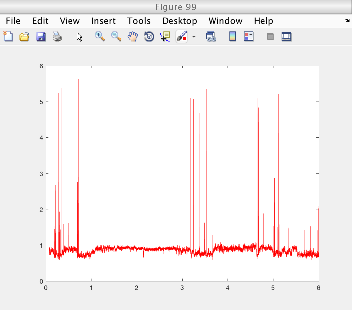
Preprocessing
As we can see from figure 99, the data contains a fair number of large outliers. Multifractal anlaysis is extremely sensitive to such large events, and we need to remove them.
We remove the ouliers in a simple way. We reject interval RR_i if:
1) RR_i is larger than 0.35 s OR RR_i is larger than 2 s
2) RR_i is more than 20% larger than the median interval on a 41 beat moving window.
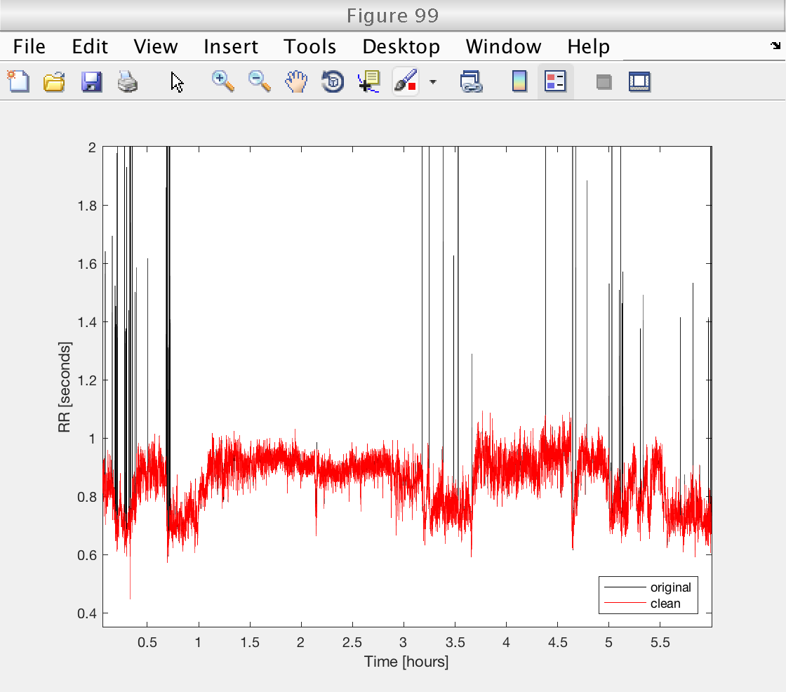
After the filtering, we interpolate the data to a uniform grid with a sampling frequency of 8 Hz, using cubic splines.
Finally, we verify the performance of the procedure on a selected record.
rr_min = 0.35;  % Smallest accepted rr_interval
rr_max = 2;     % Smallest accepted rr_interval
win_size = 41;  % Size of local median window
halfw = floor (win_size / 2);  % Half window size
fs = 8;  % Sampling frequency for interpolation
data_orig = data;

for ir = 1 : length (data)
    rr = data{ir, 2};
    t = data{ir, 1};

    % Mark intervals exceeding thresholds
    rr(rr < rr_min | rr > rr_max) = NaN;

    % Moving median filters
    for k = 1 : length (rr)
        win_beg = max (k - halfw + 1, 1);
        win_end = min (k + halfw, length (rr));
        if rr(k) > 1.2 * nanmedian (rr(win_beg : win_end));
            rr(k) = NaN;  % Mark unacceptable intervals
        end
    end

    % Remove marked
    t = t(~isnan (rr));
    rr = rr(~isnan (rr));

    % Uniform spline interpolation to target sampling frequency
    t_new = t(1) : 1 / fs : t(end);
    rr_new = interp1 (t, rr, t_new, 'spline');

    data{ir, 1} = t_new;
    data{ir, 2} = rr_new;
end

% Verify denoising on selected record
figure (99)
plot (data_orig{select, 1} / 3600, data_orig{select, 2}, 'k')
hold on
plot (data{select, 1} / 3600, data{select, 2}, 'r')
hold off
axis tight
ylim ([rr_min rr_max])
legend ({'original', 'clean'}, 'Location', 'SouthEast')
xlabel ('Time [hours]')
ylabel ('RR [seconds]')
Multifractal analysis of entire database: setup
The toolbox allows to perform the analysis of an entire database with a single command. In this case, we need to use the class 'MF_BS_tool_inter_db', where 'db' stands for database.
% Create an object of class 'MF_BS_tool_inter_db'
mo = MF_BS_tool_inter_db;

% Select which multiresolution quantities to use.
% 1: wavelet coefficients (DWT), 2: wavelet leaders (LWT)
mo.method_mrq = [1 2];

% Select the number of vanishing moments for de Daubechies wavelet
mo.nwt = 3;

% Select the statistical orders q
mo.q = [-5 -3 -2 -1 1 2 3 5];
% This will produce 10 values of q between 0.01 and 10, and then add
% their opossites also.

% Select the number of cumulants to compute
mo.cum = 2;

% Indicate starting number for figures
mo.fig_num = 100;

% Set up versbosity level.
mo.verbosity = 1;   % Number xy, with x,y either 0 or 1
                    %    x = 1: display figures
                    %    y = 1: display tables with estimates

% Select way to present results:
mo.bs_plot_type = 'superimpose';
Reader object
The tool can analyze databases in many formats, like a matrices or cell arrays with all the data, a list of files, or a directory. To have an abstract access to all these formats, it needs a 'reader' object that manage the access to the data.
In this case, since we have our data in a cell array, we need to use the function 'create_db_reader_cell' to create the proper reader.
% Select only rr_data from cell array:
rr_data = data(:, 2);

% Create reader object to read the cell array:
reader = create_db_reader_cell (rr_data);
Perform multifractal analysis
Finally, we perform the analysis by calling the analyze method with the reader we have just created.
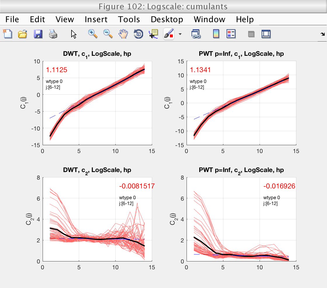
As usuall, we concentrate first on the determination of the scaling range and fractional integration order, using figures 103 and 105. Since we selected bs_plot_type = 'superimpose', we see the logscale diagrams for the individual realizations, which is useful for this task.
% Analyze the database accessed by the reader
mo.analyze (reader);

% Momentarily close figures we don't need
for f = [100, 101, 102, 104]; close(f); end
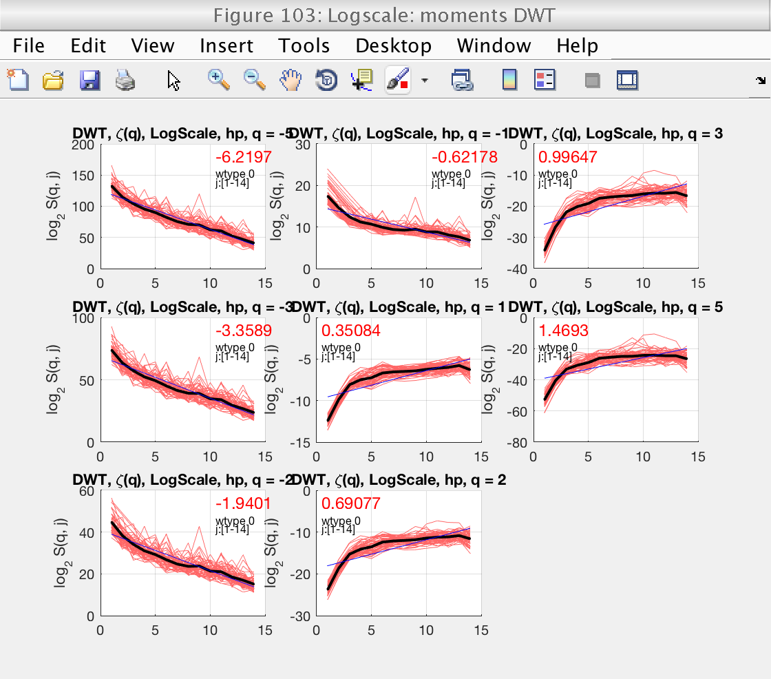
Setup scaling range:
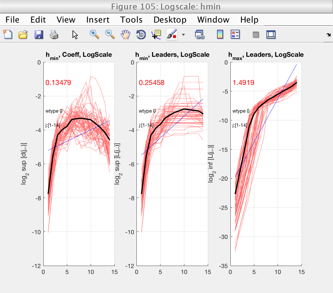
From figures 103 and 105 we see that the default scaling range is not a good choice, and that a better one would be, for instance, [6-11].
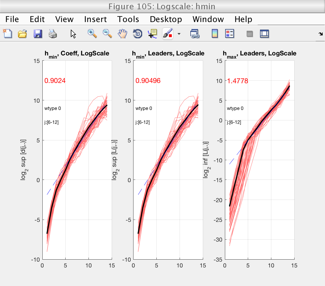
We also see that, in that scaling range, the logscale plot for h_min shows slopes around 0, both positive and negative. Just to be conservative, we will select a value of gamint = 1, equivalent to performing a full integration on the data.
We also increase the range of q, to produce smoother estimates of the spectrum.
We repeat the analysis with the new setup. We need to create a new instance of the reader, since the old one has already been exhausted.
% Adjust scaling range
mo.j1 = 6;
mo.j2 = 12;

% Adjust franctional integration
mo.gamint = 1;

% Increase range of q
mo.q = build_q_log (0.01, 10, 10);

% Analyze the data again
reader = create_db_reader_cell (rr_data);
mo.analyze (reader);

% Momentarily close figures we don't need
for f = [103, 104]; close(f); end
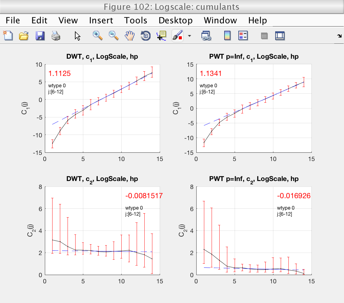
Show means and confidence intervals
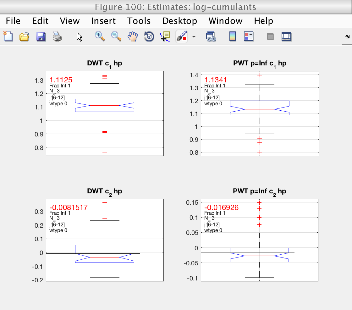
In figure 100 we see boxplots of the estimates for c1 and c2, as well as their mean (black line). They already show an interesting fact: the confidence intervals for c2 computed from LWT indicate that c2 is significantly different from 0, confirming that the data are multifractal.
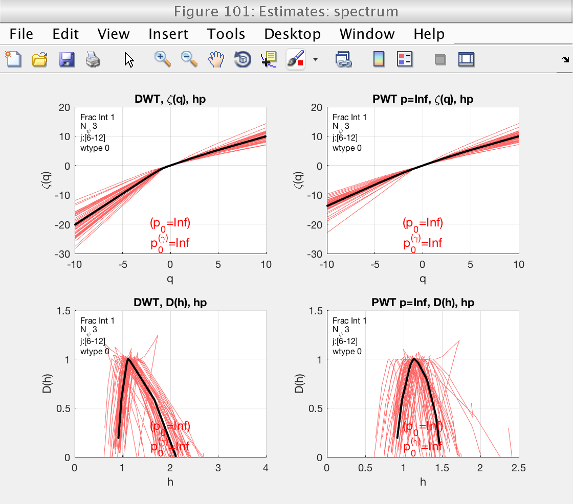
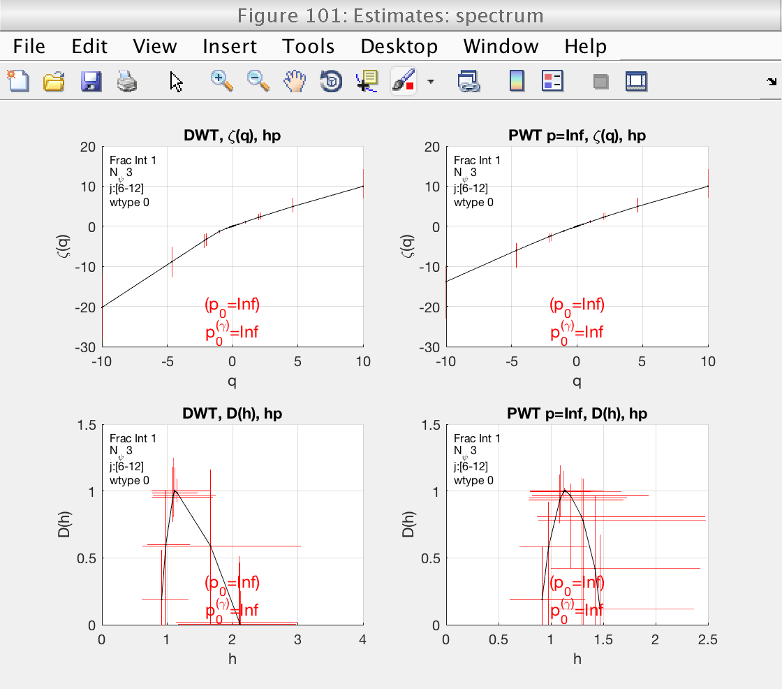
Figure 101 shows the estimates of the multifractal spectrum. However, it is difficult to visualize with the superposition of all spectra. We will change the visualization type, indicating the toolbox to show confidence intervals instead.
In this case we do not need to recompute everything. If we call
the analyze method without parameters, the tool will recreate
the plot without recomputing.
% Change visualization type to confidence intervals
mo.bs_plot_type = 'ci';

% Recreate the plots without recomputing
mo.analyze ();

% Momentarily close figures we don't need
for f = [100, 103, 104, 105]; close(f); end
Scatter plots of results
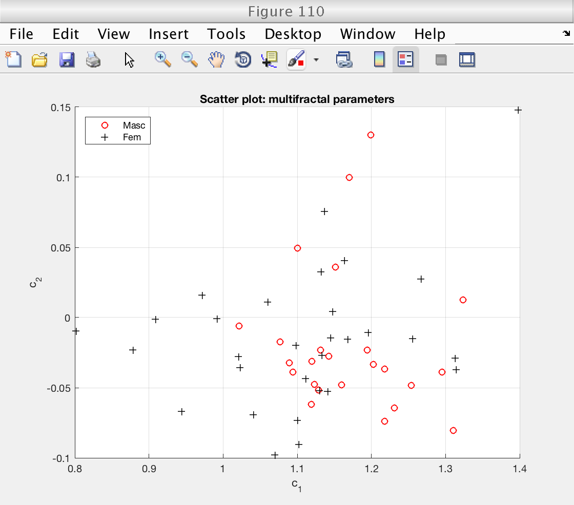
Finally, we create a scatter plot with the multifractal parameters c1 and c2.
The mean estimates are stored in field mo.est.LWT.t, and the individual estimates of each signals are stored in mo.est.LWT.BS.T.
As usual, both fields contain all the estimates: zeta(q), D(q), h(q) and cp. To extract only the log-cumulants, we use the get_cid function to get the corresponding indices.
There doesn't seem to be a large structure on the scatter plot.
% Get indices for log cumulants
cid = mo.get_cid ();

% Access mean estimates
cp_mean = mo.est.LWT.t(cid);

% Access individual estimates for each signal
cp_all = mo.est.LWT.BS.T(:, cid);

% Load gender grouping variables as logical values:
gender = load ('genders_binary.txt');  % 0: feminin, 1: masculin
gender = logical (gender);

% Create scatter plot
figure (110)
% Plot feminine subjects
scatter (cp_all(~gender, 1), cp_all(~gender, 2), 'ro')
hold on
% Plot masculine subjects
scatter (cp_all(gender, 1), cp_all(gender, 2), 'k+')
hold off
grid on
xlabel ('c_1')
ylabel ('c_2')
title ('Scatter plot: multifractal parameters')
legend ('Masc', 'Fem', 'Location', 'NorthWest')
Classify using k-NearestNeighbors
As an illustration, we attempt to predict gender based on multifractal attributes.
We use a simple k-NearestNeighbors classifier. We use multifractal parameters  and
and  (columns of variable cp_all) as predictors, and the gender as response.
% Train classifier using 11 neighbours, and 5-fold cross-validation
knn_model = fitcknn(cp_all, gender, ...
                    'NumNeighbors', 11, 'Standardize', 1, 'kFold', 10);

% Measure classification accuracy:
accuracy = 1 - knn_model.kfoldLoss ();

fprintf ('Accuracy: %g\n', accuracy)
Accuracy: 0.703704