Multifractal analysis using MF_BS_tool

Tutorial demo on the use of MF_BS_tool for multifractal analysis.

This demo will teach the basic concepts of the toolbox, as well as the two main steps of practical multifractal analysis: the selection of the scaling range and of the order of fractional integration.

Roberto Leonarduzzi, Patrice Abry

June 2018

Contents

Set up the path

Add root folder of toolbox to path (subfolders will be added automatically)

addpath ~/Documents/code/mf_bs_tool

Load example data

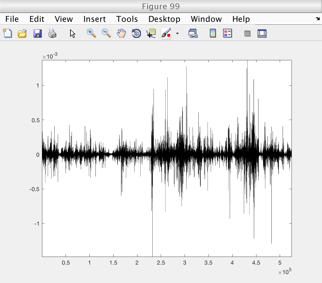
% Load data and theoretical multifractal spectrum:
load ('data_example_1.mat', 'data', 'D_theo', 'h_theo', 'q_theo', 'zq_theo', 'c_theo')

% Plot the data to  get a first impression
figure (99)
plot (data, 'k')
axis tight

Multifractal analysis: setup

The interface to the multifractal analysis toolbox is provided by an object of class 'MF_BS_tool_inter'. This object contains all the parameters to control the analysis, as well as the main routine to perform it.

We will create an object and set up its basic parameters.

% Create an object of class MF_BS_tool_inter
mo = MF_BS_tool_inter;

% Select which multiresolution quantities to use.
% 1: wavelet coefficients (DWT), 2: wavelet leaders (LWT)
mo.method_mrq = [1 2];

% Select the number of vanishing moments for de Daubechies wavelet
mo.nwt = 3;

% Select the statistical orders q
mo.q = [-5 -3 -2 -1 1 2 3 5];
% This will produce 10 values of q between 0.01 and 10, and then add
% their opossites also.

% Select the number of cumulants to compute
mo.cum = 2;

% Indicate starting number for figures
mo.fig_num = 100;

% Set up versbosity level.
mo.verbosity = 1;   % Number xy, with x,y either 0 or 1
                    %    x = 1: display figures
                    %    y = 1: display tables with estimates

Multifractal analysis: default parameters

We will perform a first analysis using the default parameters proposed by the tool.

The tool will produce a series of figures showing:

0) Estimates of log cumulants (for DWT and LWT)

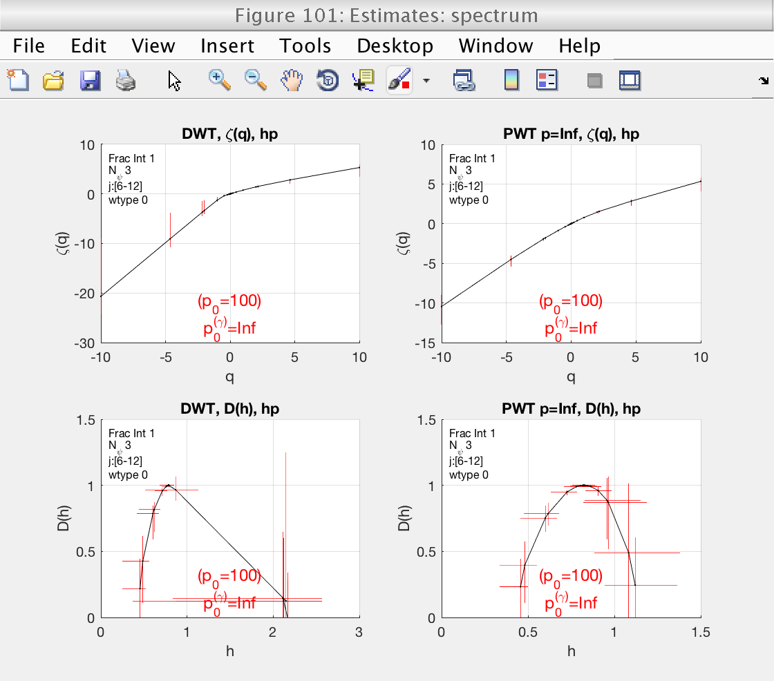
1) Estimates for zeta(q) and D(h) (for DWT and LWT)

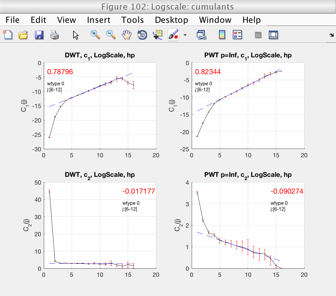
2) Loglog plots and linear fits of cumulants (for DWT and LWT)

3) Loglog plots and linear fits of structure functions for DWT

4) Loglog plots and linear fits of structure functions for LWT

5) Loglog plots of and linear fits largest and smallest coefficients

We will start by focusing on figure 103.

% To analyze the data, we call the 'analyze' method.
% The input can be a 1d or 2d array.
mo.analyze (data);

% Momentarily close figures we don't need
for f = [100, 101, 102, 104, 105]; close(f); end

IMPORTANT

Before looking at the estimates of the multifractal spectrum, two things need to be verified: 1) That the scaling range is correct, and the linear fits are reasonable. 2) That the condition h_min > 0 holds. Wavelet leaders are defined only when h_min > 0. If the condition doesn't hold, the estimates obtained with wavelet leaders will be extremely biased and should not be used.

These two things are related, since to estimate h_min we need to do a linear regression with a correct scaling range.

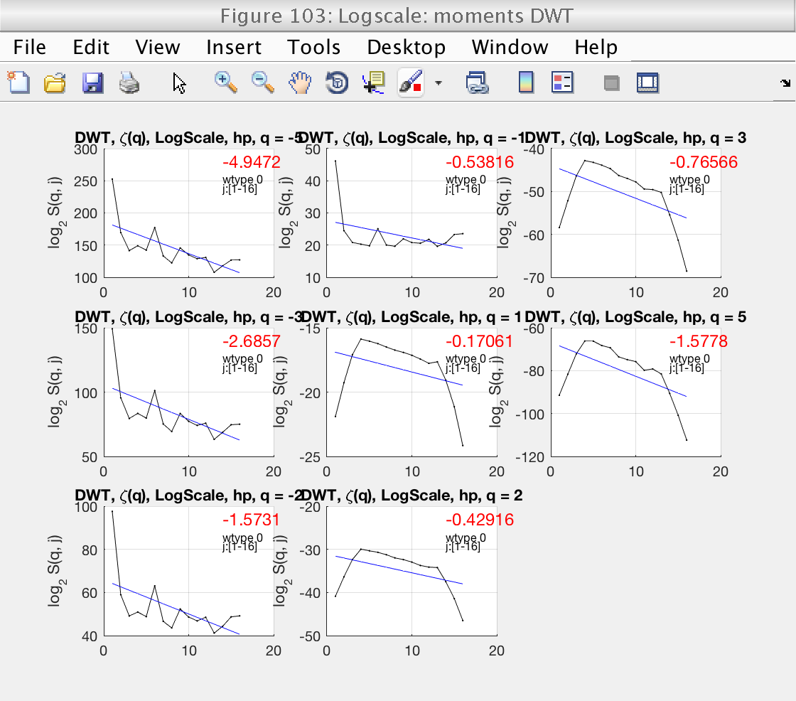
Scaling range selection: wavelet coefficients

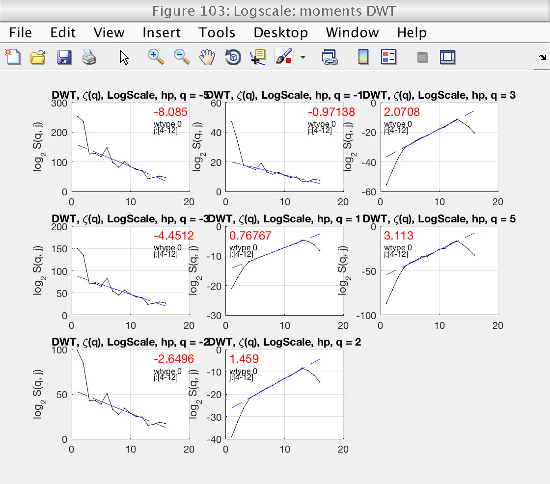
We start by looking at Fig 103, which shows the loglog plots with wavelet coefficients for different values of q. The plots can be enlarged by clicking on them. For DWT, we should consider positive values of q only. Looking at these plots, we see that the default scaling range [1, 18] is not correct: the linear fits (blue lines) do not fit well the structure functions (black lines).

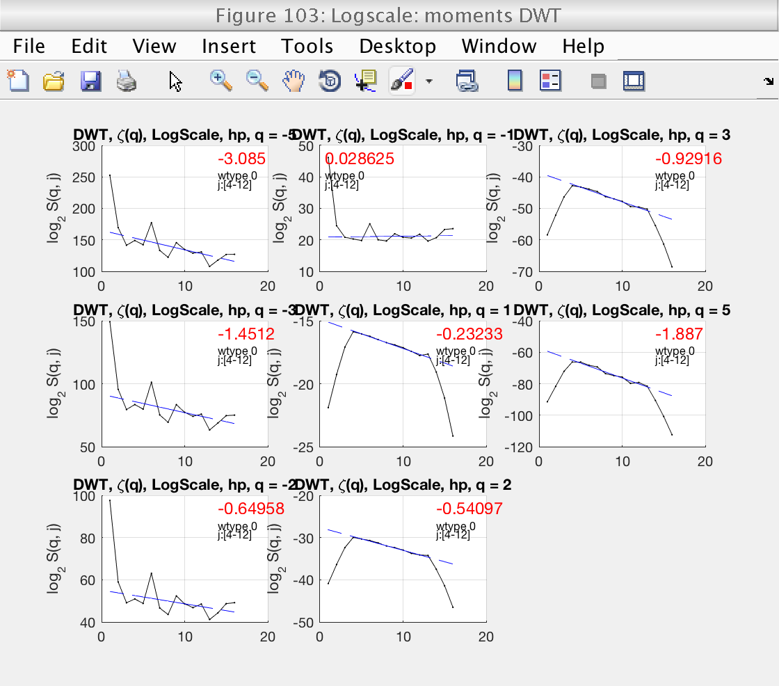
We select the more reasonable scaling range [4, 12] by setting the properties j1 and j2:

A new inspection of figure 103 shows that the scaling range is satisfactory.

mo.j1 = 4;
mo.j2 = 12;
mo.analyze (data);

% Momentarily close figures we don't need
for f = [100, 101, 102, 104]; close(f); end

Estimation of h_min and integration

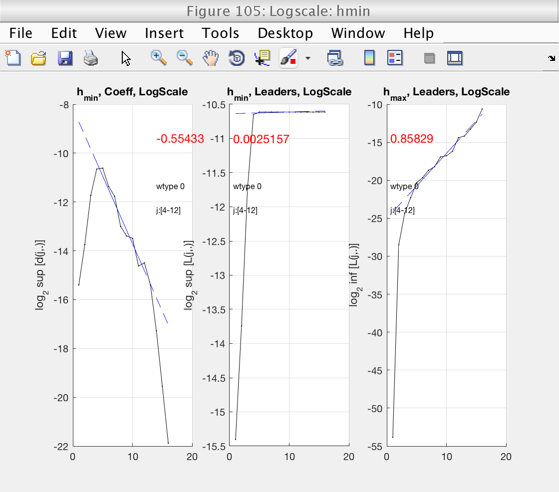
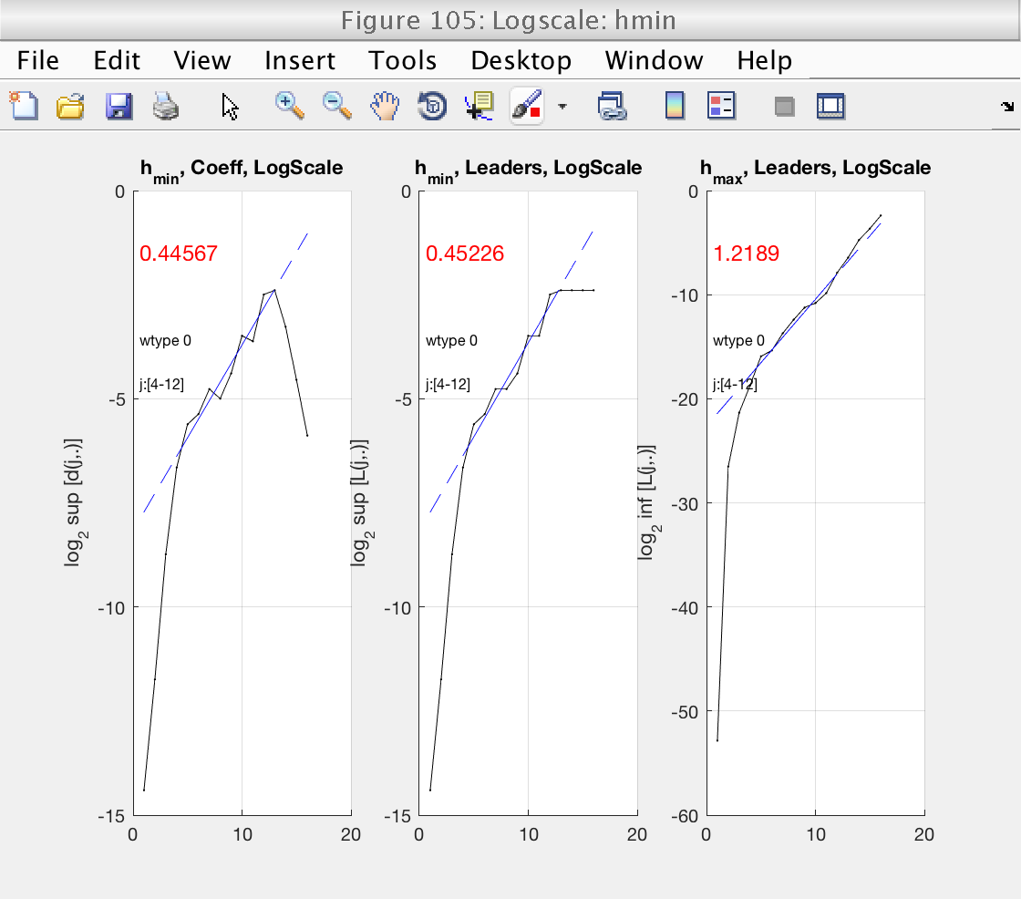
Now that the scaling range is correct, we turn our attention to the estimation of h_min. This is shown in Fig 6, left panel. h_min is provided by the slope of the linear fit in this plot. The value of the slope is shown in red numbers.

We see that h_min = -0.55 < 0, meaning that the minimum regularity does not hold and can not use wavelet leaders. The problem with leaders is illustrated in the middle panel. Under normal circumstances, the left and middle pannels should be similar. In this case, however, wavelet leaders are almost constant and have a slope of 0. This is the signature of problems with the minimum regularity condition.

To solve these problems, we need to increase the regularity of our data by integrating it. The toolbox provides a way to do this through the gamint property: it will perform a fractional integration of order gamint.

We need to select a value satisfying gamint > h_min. To be on the safe side, we will select gamint = 1 > 0.55.

Now we see that h_min is positive, and that the left and middle plots (DWT and leaders) have a similar behavior.

In this situation, we are confident that our leaders are well defined and unbiased.

mo.gamint = 1;
mo.analyze (data);

% Momentarily close figures we don't need
for f = [100, 101]; close(f); end

Scaling range selection: wavelet leaders

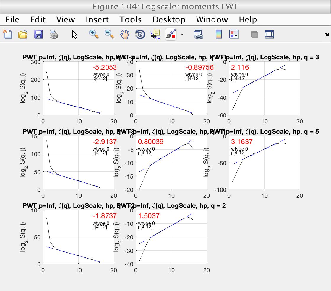
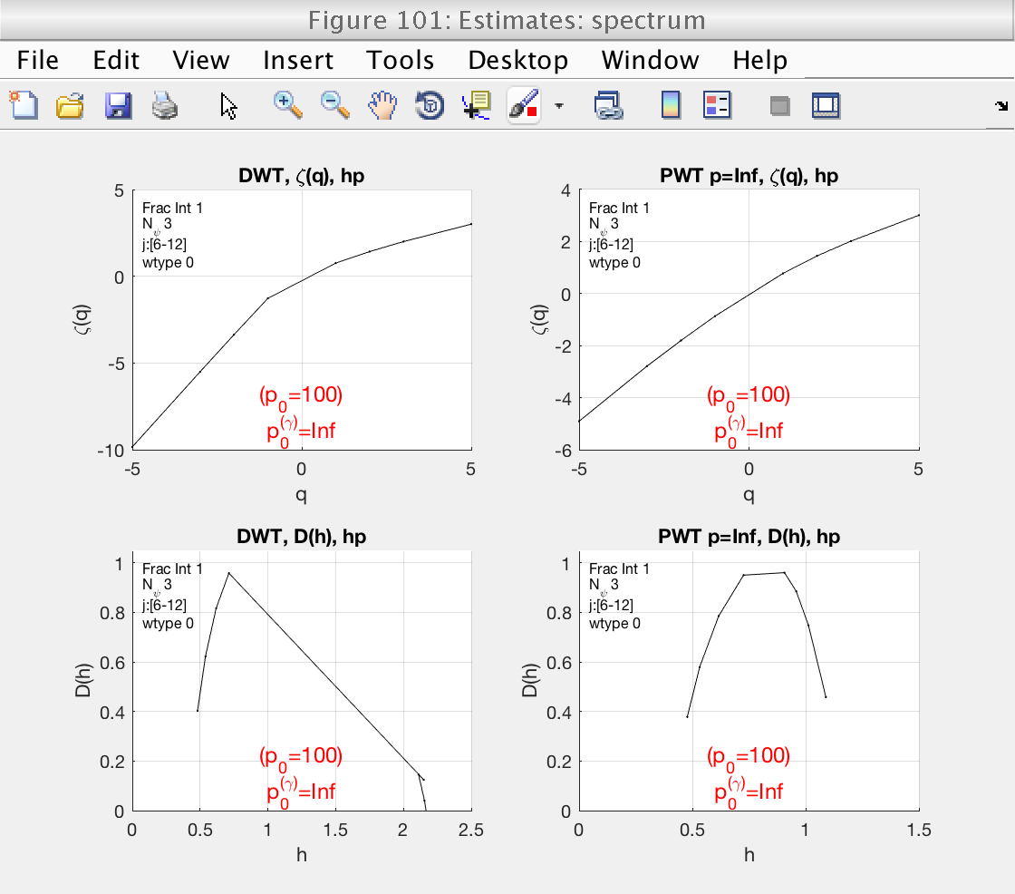
Now that wavelet leaders are computed correctly, we can verify that the scaling range is correct for wavelet leaders as well. We do this by looking at figure 105. Now that we are looking at wavelet leaders we can also consider negative values of q.

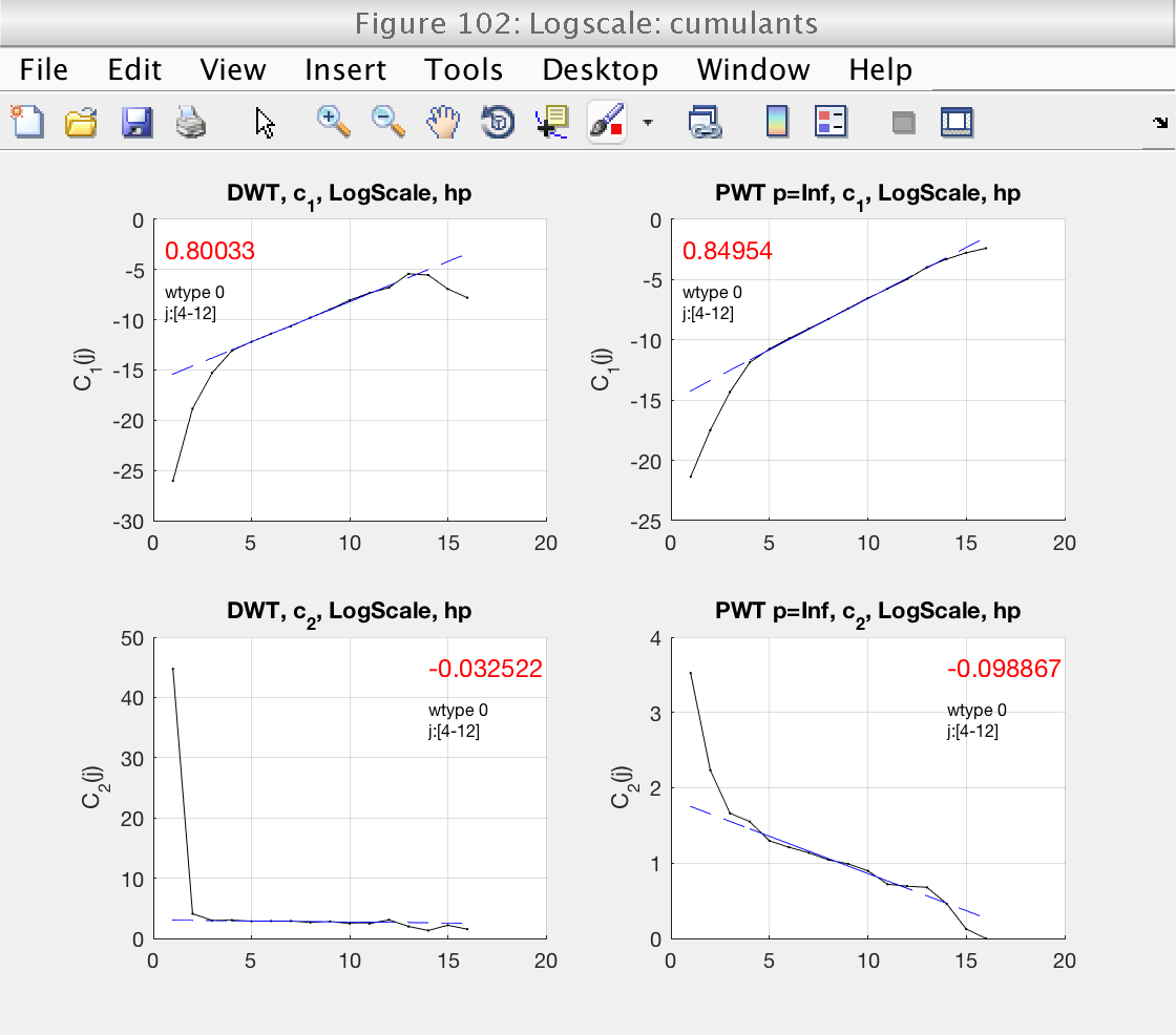
Finally, we should also check that the scaling range is correct in the loglog plots for the cumulants (Fig 3).

From all these plots, we can refine our scaling range before looking at the final estimates of the multifractal spectrum in Fig. 102.

mo.j1 = 6;
mo.j2 = 12;
mo.analyze (data);

% Momentarily close figures we don't need
for f = [100, 102, 103, 104, 105]; close(f); end

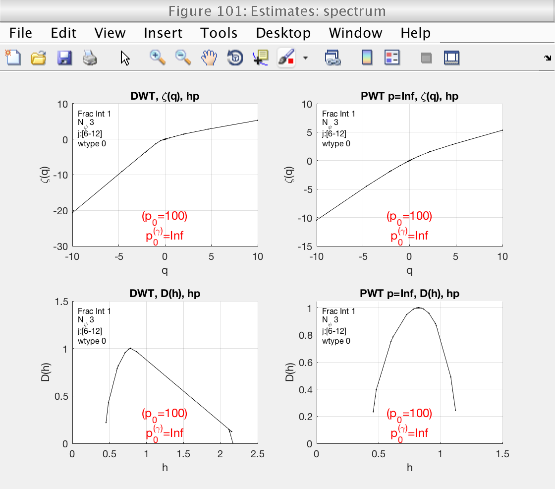
Selection of the orders q

To improve the estimation of the multifractal spectrum around its maximum, we can refine the statistical orders q that are used.

The toolbox provides the utility function build_q_log to provide a nice array of values of q that are logarithmically spaced:

mo.q = build_q_log (0.01, 10, 10);
mo.analyze (data);

% This will produce 10 values of q between 0.01 and 8, and then add
% their opossites also.

% Momentarily close figures we don't need
for f = [100, 102, 103, 104, 105]; close(f); end

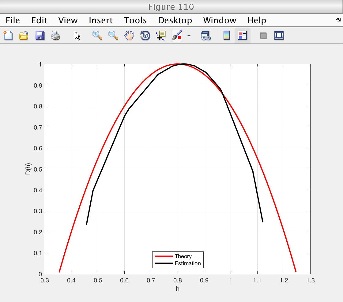
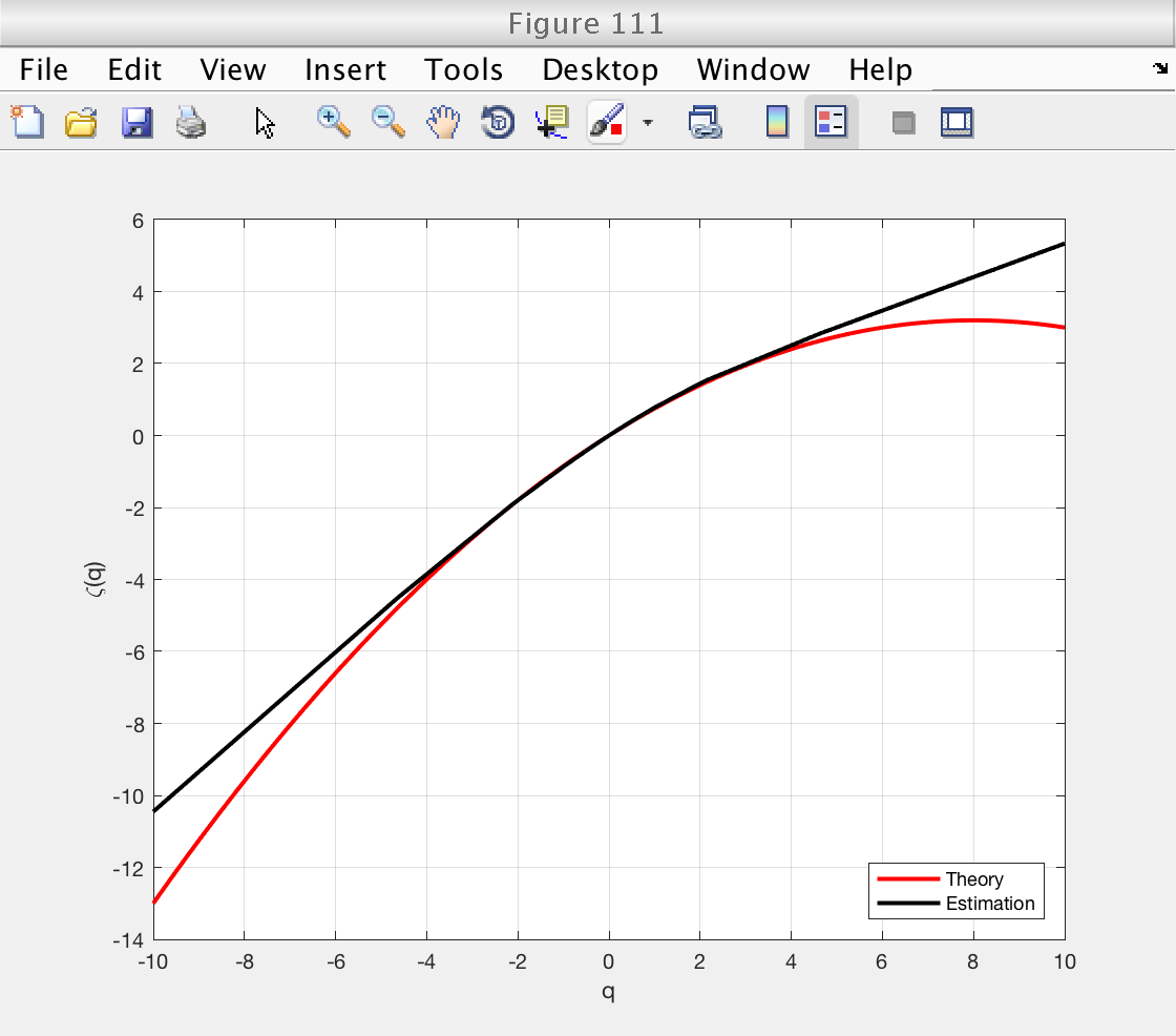
Multifractal spectrum: theory vs estimation

Now we illustrate how to recover the estimates. We will plot the theoretical spectrum and superimpose the esimated spectrum and scaling function.

We already loaded the variables 'h_theo' and 'D_theo' from the example file.

We can recover all the esimates stored in the mo object by doing:

estimates = mo.est.LWT.t;

% This array contains all the estimates: [zeta(q), D(q), h(q), c_m]
% We can get the indices of each individual estimate by using the
% following methods:
z_index = mo.get_zid ();  % Indices of zeta(q)
h_index = mo.get_hid ();  % Indices of h(q)
D_index = mo.get_Did ();  % Indices of D(q)
c_index = mo.get_cid ();  % Indices of c_p

% And now we can get the individual estimates:
zq = estimates(z_index);  % Estimates of zeta(q)
hq = estimates(h_index);  % Estimates of h(q)
Dq = estimates(D_index);  % Estimates of D(q)
cp = estimates(c_index);  % Estimates of c_p

% Now we can make the desired figures:
figure (110)
plot (h_theo, D_theo, 'r', 'Linewidth', 2)
hold on
plot (hq, Dq, 'k', 'Linewidth', 2)
hold off
grid on
xlabel ('h')
ylabel ('D(h)')
legend ('Theory', 'Estimation', 'Location', 'South')

figure (111)
plot (q_theo, zq_theo, 'r', 'Linewidth', 2)
hold on
plot (mo.q, zq, 'k', 'Linewidth', 2)
hold off
grid on
xlabel ('q')
ylabel ('\zeta(q)')
legend ('Theory', 'Estimation', 'Location', 'SouthEast')

Bootstrap-based confidence intervals

The tool also allows to show bootstrap-based confidence intervals on all estimates. To activate them, we set the number of bootstrap resamples to a value larger than 0.

We will use this information to display the estimates of the log-cumulants and theor corresponding confidence inervals.

% Set the number of bootstrap resamples:
mo.n_resamp_1 = 50;

% Activate the computation of confidence intervals for the estimates:
mo.CI = 1;

% Select the type of confidence interval (more than 1 can be chosen):
mo.ci_method = [1 2 3];  % 1: Normal; 2: Basic; 3: Percentile

% Analyze the data again (it will take some time):
mo.analyze (data)

% Momentarily close figures we don't need
for f = [ 103, 104, 105]; close(f); end

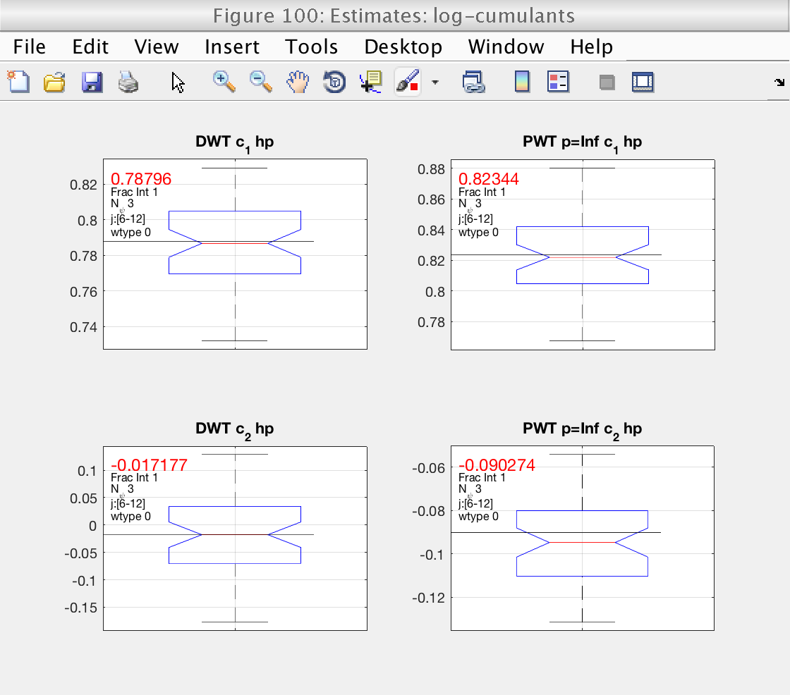
Display cumulants and confidence intervals

% Get basic confidence intervals for the log-cumulants:
method_index = 2;

for ic = 1 : mo.cum  % Loop log-cumulants
    cp_ci(ic, 1) = mo.stat.LWT.confidence{c_index(ic)}{method_index}.lo;
    cp_ci(ic, 2) = mo.stat.LWT.confidence{c_index(ic)}{method_index}.hi;
end

fprintf ('     %5s %10s    %10s\n', 'Theory', 'Estimation', 'Confidence Interval')
for ic = 1 : mo.cum
    fprintf ('c%i: %5.3g  %10.3g    [%7.3g  %7.3g]\n', ic, c_theo(ic), cp(ic), cp_ci(ic, :));
end

     Theory Estimation    Confidence Interval
c1:   0.8       0.823    [  0.767    0.879]
c2:  -0.1     -0.0903    [ -0.126  -0.0491]

Published with MATLAB® R2016a