Self-similar analysis using MF_BS_tool

Tutorial demo on the use of MF_BS_tool for the analysis of self-similar processes.

This demo will teach the basic elements to use the toolbox.

The toolbox can be downloaded from:

http://www.ens-lyon.fr/PHYSIQUE/Equipe3/Multifractal/software.html

Roberto Leonarduzzi, Patrice Abry

June 2018

Set up the path
Load example data
Self-similar analysis: setup
Multifractal analysis: default parameters
Scaling range selection: wavelet coefficients
Confidence intervals
Hurst exponent: theory vs estimation
Access to logscale diagrams
Equivalence of scales and frequencies
Comparison with Fourier spectrum

Set up the path

Add root folder of toolbox to path (subfolders will be added automatically)

addpath ~/Documents/code/mf_bs_tool

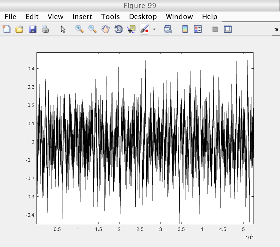
Load example data

% Load data and theoretical multifractal spectrum:
load ('data_example_ss.mat', 'data', 'H_theo') ;
% nbsamples = 2^18 ; H_theo = 0.3 ; [data,x] = synthfbmcircul(nbsamples,H_theo) ;

% Plot the data to  get a first impression
figure (99)
plot (data, 'k')
axis tight

Self-similar analysis: setup

The interface to the multifractal analysis toolbox is provided by an object of class 'MF_BS_tool_inter'. This object contains all the parameters to control the analysis, as well as the main routine to perform it.

We will create an object and set up its basic parameters.

For the analysis of self-similar processes we will only use wavelet coefficients and second-order statistics.

% Create an object of class MF_BS_tool_inter
mo = MF_BS_tool_inter;

% Select which multiresolution quantities to use.
% 1: wavelet coefficients (DWT), 2: wavelet leaders (LWT)
mo.method_mrq = [1];

% Select the number of vanishing moments for de Daubechies wavelet
mo.nwt = 3;

% Select the statistical orders q
mo.q = [2];
% This will produce 10 values of q between 0.01 and 10, and then add
% their opossites also.

% Indicate starting number for figures
mo.fig_num = 100;

% Set up versbosity level.
mo.verbosity = 1;   % Number xy, with x,y either 0 or 1
                    %    x = 1: display figures
                    %    y = 1: display tables with estimates

Multifractal analysis: default parameters

We will perform a first analysis using the default parameters proposed by the tool.

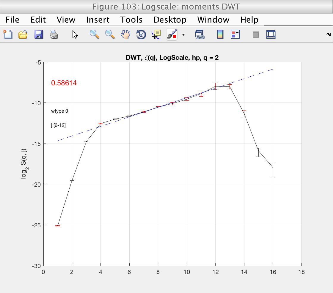
The tool will produce many figures showing several estimates. For this demo, we will concentrate only on figure 103, which shows the logscale diagrams for wavelet coefficients.

% To analyze the data, we call the 'analyze' method.
% The input can be a 1d or 2d array.
mo.analyze (data);

% Momentarily close figures we don't need
for f = [100, 101, 102, 105]; close(f); end

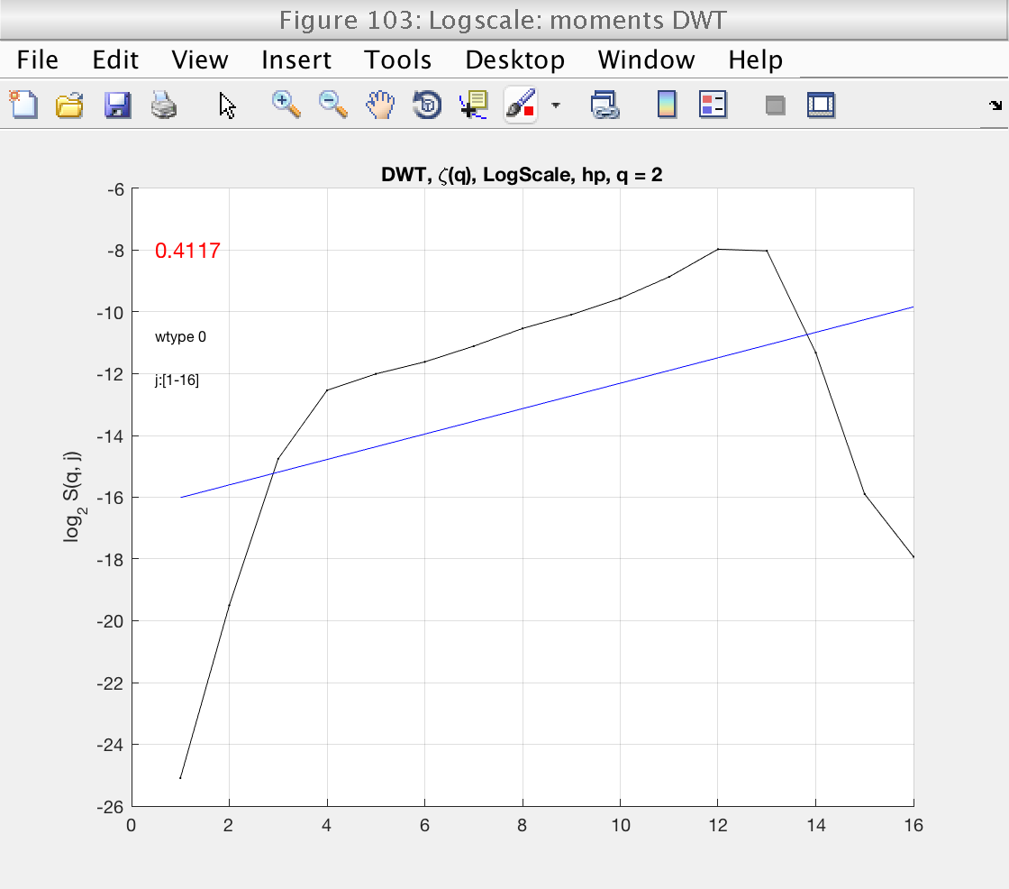
Scaling range selection: wavelet coefficients

We start by looking at Fig 103, which shows the loglog plot for wavelet coefficients, and the estimate of the slope in red. The value of the slope is 2H.

Looking at the plot, we see that the default scaling range [1, 18] is not correct: the linear fit (blue line) does not fit well the structure function (black line).

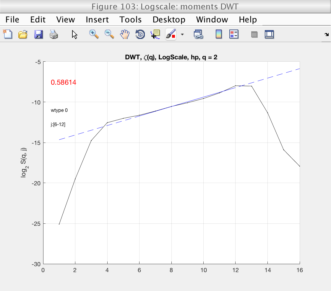
We select the more reasonable scaling range [4, 12] by setting the properties j1 and j2:

A new inspection of figure 103 shows that the scaling range is satisfactory.

mo.j1 = 6;
mo.j2 = 12;
mo.analyze (data);

% Momentarily close figures we don't need
for f = [100, 101, 102, 105]; close(f); end

Confidence intervals

The tool also allows to show bootstrap-based confidence intervals on all estimates. To activate them, we set the number of bootstrap resamples:

% Set the number of bootstrap resamples:
mo.n_resamp_1 = 100;

% Activate the computation of confidence intervals for the estimates:
mo.CI = 1;

% Select the type of confidence interval (more than 1 can be chosen):
mo.ci_method = [1 2 3];  % 1: Normal; 2: Basic; 3: Percentile

% Analyze the data again:
mo.analyze (data)

% Momentarily close figures we don't need
for f = [100, 101, 102, 105]; close(f); end

Hurst exponent: theory vs estimation

Now we illustrate how to recover the estimates. We will compare the theoretical and estimated spectra.

We already loaded the variable 'H_theo' from the example file.

% Index of estimates for H:
id_H = 1;
% (We access the first position because there is only one value of q)

% Get estimate for H
H_est = mo.est.DWT.t(1) / 2;

% Get basic confidence intervals for H
id_method = 2;
ci_H(1) = mo.stat.DWT.confidence{id_H}{id_method}.lo / 2;
ci_H(2) = mo.stat.DWT.confidence{id_H}{id_method}.hi / 2;


fprintf('\nEstimation of H:\n')
fprintf ('Theoretical H = %g\n', H_theo)
fprintf ('Estimated   H = %g [%g, %g]\n', H_est, ci_H)

Estimation of H:
Theoretical H = 0.3
Estimated   H = 0.29307 [0.274958, 0.317817]

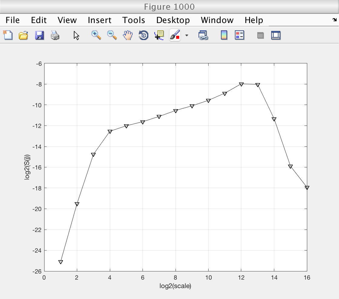
Access to logscale diagrams

We now reproduce figure 103 to show how to access the logscale diagrams stores in the object

figure (1000)
plot (mo.logstat.DWT.est(1,:), 'vk-')
grid on
xlabel('log2(scale)');
ylabel('log2(S(j))');

Equivalence of scales and frequencies

Finally, we show the frequency ranges covered by each wavelet scale:

fs = 1;  % sample frequency
j = [1 : length(mo.logstat.DWT.scale)];  % octaves
f_high    = fs * 2.^(-j);
f_low     = fs * 2.^(-(j + 1));
f_central = fs * 2.^(-j) * 3 / 4 ;

fprintf ('\nEquivalence of scales and frequencies:\n')
fprintf ('%s %10s %10s %10s\n', 'Scale', 'f_high', 'f_central', 'f_low')
fprintf ('%5i %10.3g %10.3g %10.3g\n', [j ; f_high ; f_central ; f_low])

Equivalence of scales and frequencies:
Scale     f_high  f_central      f_low
    1        0.5      0.375       0.25
    2       0.25      0.188      0.125
    3      0.125     0.0938     0.0625
    4     0.0625     0.0469     0.0312
    5     0.0312     0.0234     0.0156
    6     0.0156     0.0117    0.00781
    7    0.00781    0.00586    0.00391
    8    0.00391    0.00293    0.00195
    9    0.00195    0.00146   0.000977
   10   0.000977   0.000732   0.000488
   11   0.000488   0.000366   0.000244
   12   0.000244   0.000183   0.000122
   13   0.000122   9.16e-05    6.1e-05
   14    6.1e-05   4.58e-05   3.05e-05
   15   3.05e-05   2.29e-05   1.53e-05
   16   1.53e-05   1.14e-05   7.63e-06

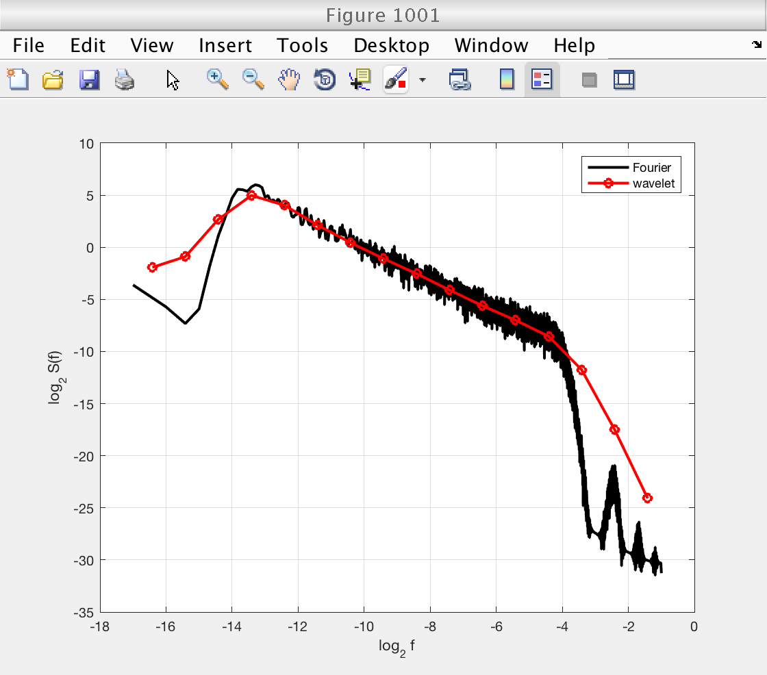
Comparison with Fourier spectrum

We can also compare the wavelet and Fourier spectra. For this, we plot the wavelet spectrum as a function of frequency instead of scale. We also need to change the normalization used by the toolbox's wavelet transform.

The function wavelet_fourier_spectrum, provided by the toolbox, computes a Welch periodogram and a wavelet spectrum with the correct normalization, as a function of frequency.

% Window size for Welch periodogram
window_size = length (data) / 4;

% Sampling frequency
fs = 1;

% Compute both spectra.
[S_fou, f_fou, S_wav, f_wav] = wavelet_fourier_spectrum (data, mo.nwt, window_size, fs, 0);

figure (1001)
plot (log2 (f_fou), log2 (S_fou), 'k', 'LineWidth', 2)
hold on
plot (log2 (f_wav), log2 (S_wav), 'ro-', 'LineWidth', 2)
hold off
grid on
xlabel ('log_2 f')
ylabel ('log_2 S(f)')
legend ('Fourier', 'wavelet', 'Location', 'NorthEast')