Sparse classification and, cross-validation

Tutorial demo on the use of sparse Suppor Vector Machines and cross validation.

Classiffication is done on a modified version of Ripley's data set.

The performance of classical and sparse SVMs are compared. Training, testing and cross-validated errors are compared.

Roberto Leonarduzzi, Patrice Abry

June 2018

Setup path and random number generator
Generate Ripley's dataset
Visualize features
Setup Sparse SVM
Setup Classical SVM
Classification: training and testing set
Cross-validation
Performance measurement
Figures: performance
Select optimal sparsity
Figures: weights

Setup path and random number generator

We add the folders with the tools for cross-validation and sparse SVM to the path.

For reproducibility, we fix the seed of the random number generator

addpath ~/Documents/code/classif_tools/cross_validate/
%addpath ~/Dropbox/postdoc/classif/cross_validate/
addpath ./SparseSVM/

% Fix stream of random numbers, for reproducibility
s1 = RandStream.create('mrg32k3a','Seed', 10);
s0 = RandStream.setGlobalStream(s1);

Generate Ripley's dataset

Ripley's dataset consists of features from a mixture of two bidimensional normal distributions with different means and the same variance.

Features from class 1 come from a mixture of gaussians with means $\mu_{11}=(0.4, 0.7)$ and $\mu_{12}=(-0.3, 0.7)$ .

Features from class 2 come from a mixture of gaussians with means 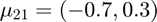$\mu_{21}=(-0.7, 0.3)$ and $\mu_{22}=(0.3, 0.3)$ .

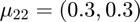We further repeat these bidiminensional features K times, for a total of 2K initial Ripley features.

To these initial features, we add two types of new features:

1) correlated features obtained by summing random pairs of the initial features, and corrupting them with random Gaussian noise.

2) random features.

These new features are not discriminant, and make the classification problem more difficult.

% Number of samples on each class, for training and testing
n1_train = 500;
n2_train = 500;
n1_test  = 100;
n2_test  = 100;

% Number of featurs of each type:
K  =  5 ; % Number of copies of Ripley features
KC = 45 ; % number of correlated features
KN = 40;  % number of random features

% Variance of initial features:
sigma = 0.2;

% Generate initial Ripley's dataset
[X_train, y_train] = generateRipley (n1_train, n2_train, 2 * K, sigma);
[X_test , y_test ] = generateRipley (n1_test , n2_test , 2 * K, sigma);

% Create correlated features
X_train = correlate_features (X_train, KC, 0.8 * sigma);
X_test  = correlate_features (X_test , KC, 0.8 * sigma);

% Create random features:
X_train = [X_train , randn(n1_train + n2_train, KN)];
X_test  = [X_test  , randn(n1_test  + n2_test , KN)];

% Convert output labels from {-1, 1} to {1, 2}
y_train = (y_train + 3) / 2;
y_test = (y_test + 3) / 2;

% Identify which label will be the "positive" class:
pos_class = 2;

% Normalize features: zero mean and unit variance
X_train = zscore (X_train, 1);
X_test  = zscore (X_test , 1);

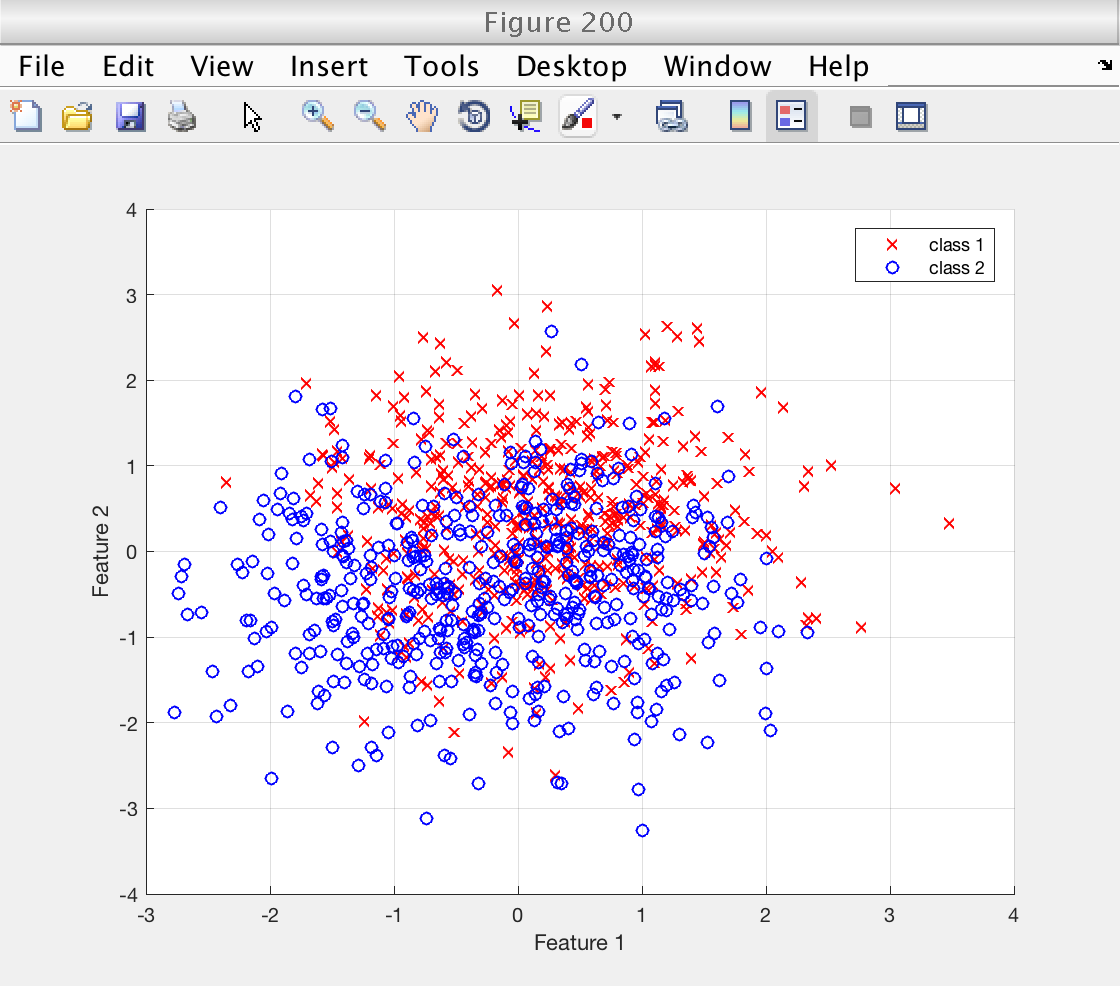
Visualize features

We visualize the first two features: the first of the K repetitions of the bidimensional Ripley features.

The classes appear highly mixed due to the relatively large standard deviation sigma that was chosen for the synthesis.

We will see that, despite this, a relatively high classification performance is achieved using SVMs.

figure (200)
idx = 1 : n1_train;  % indices of first class
scatter (X_train(idx, 1), X_train(idx, 2), 'rx')
hold on
idx = n1_train + (1 : n2_train);
scatter (X_train(idx, 1), X_train(idx, 2), 'bo')
hold off
grid on
xlabel ('Feature 1')
ylabel ('Feature 2')
legend ('class 1', 'class 2')

Setup Sparse SVM

We use a wrapper for our SparseRegularizedSVM_train function. We specify the tolerance and maximum number of iterations. Our wrapper receives also a sparsity level.

The training wrapper will return 2 outputs: the weights and the bias.

The test wrapper returns the labels and the scores.

% Sparsity levels for SSVM
ssvm_sp_vec = 2 .^ ([-9 : -1]);

% Define standard training and testing functions:
train_fun_ssvm = @(data, y, sp) ...
    ssvm_train_wrapper (data, y, sp, 'eps', 1e-9, 'maxiter', 1e6);
test_fun_ssvm = @ssvm_test_wrapper;

% Indicate number of outputs of the training function
nout_train_ssvm = nargout (@ssvm_train_wrapper);

Setup Classical SVM

We use a wrapper for matlab's fitcsvm function. We use a cell array to include the parameters we will use; in this case, we select a linear kernel.

The training wapper will return 3 outputs: the weights, the bias, and an SVM model.

The test wrapper returns the labels and the scores.

A small detail: we need to add a bogus parameter to our training function to handle the grid of parameters cross_validate will attempt to use. However, we will never use this parameter explicitly, so we can forget about it.

% Parameters for Matlab's SVM function
svm_params = {'KernelFunction', 'linear'};

% Define standard training and testing functions. Add bogus parameter to for
% cross_validate's grid.
train_fun_csvm = @(data, y, bogus) ...
    classic_svm_train_wrapper (data, y, svm_params);
test_fun_csvm = @classic_svm_test_wrapper;

% Indicate number of outputs of the training function
nout_train_csvm = nargout (@classic_svm_train_wrapper);

Classification: training and testing set

Train and measure performance in training and testing set

We do the classification with SSVM for each sparsity level, and only once for classical SVM.

% Sparse SVM: classification for each sparsity level
for is = 1 : length (ssvm_sp_vec)  % loop sparsity
    fprintf ('Sparsity %g -- ', ssvm_sp_vec(is))
    tic

    % Reserve output of right size:
    out = cell (1, nout_train_ssvm);

    % Train classifier:
    [out{:}] = train_fun_ssvm (X_train, y_train, ssvm_sp_vec(is));

    % Compute training error:
    [yhat_train_ssvm(is, :), score_train_ssvm(is, :)] = ...
        test_fun_ssvm(X_train, y_train, out{:});

    % Compute testing error:
    [yhat_test_ssvm(is, :), score_test_ssvm(is, :)] = ...
        test_fun_ssvm(X_test, y_test, out{:});

    % Store weights
    weights_ssvm(is, :) = out{1};

    toc
end

% Classical SVM: clasification
% Reserve output of right size:
out = cell (1, nout_train_csvm);

% Train classifier:
[out{:}] = train_fun_csvm (X_train, y_train);

% Compute training error:
[yhat_train_csvm, score_train_csvm] = ...
    test_fun_csvm(X_train, y_train, out{:});

% Compute testing error:
[yhat_test_csvm, score_test_csvm] = ...
    test_fun_csvm(X_test, y_test, out{:});

% Store weights
weights_csvm = out{1};

Sparsity 0.00195312 -- Elapsed time is 0.290624 seconds.
Sparsity 0.00390625 -- Elapsed time is 0.341281 seconds.
Sparsity 0.0078125 -- Elapsed time is 0.424938 seconds.
Sparsity 0.015625 -- Elapsed time is 0.606583 seconds.
Sparsity 0.03125 -- Elapsed time is 0.787019 seconds.
Sparsity 0.0625 -- Elapsed time is 1.083927 seconds.
Sparsity 0.125 -- Elapsed time is 1.295806 seconds.
Sparsity 0.25 -- Elapsed time is 1.580282 seconds.
Sparsity 0.5 -- Elapsed time is 1.778901 seconds.

Cross-validation

We train and meassure performance again, this time using cross-validation.

The cross_validate function receives the training data and the training and testing functions and performs K-fold cross-validation on a grid of parameters (5th argument).

The function returns the cross-validated estimates of the weights, labels and scores, for each point of the grid. Estimates for the weights are averages over all the folds.

We set the number of folds we use. Also, we set the number of times the cross-validation is repeated to reduce the sampling bias.

% Parameters for cross-validation
num_fold = 10;  % Number of folds
num_rep = 1;    % Number of repetitions

% Perform cross validation on SSVM
param_grid = {ssvm_sp_vec};  % Use grid of sparsity levels
[weights_cv_ssvm, yhat_cv_ssvm, score_cv_ssvm] = ...
    cross_validate (train_fun_ssvm, test_fun_ssvm, X_train, y_train, param_grid, ...
                    'verbose', true, 'num_fold', num_fold, ...
                    'num_rep', num_rep, 'num_outputs_train', nout_train_ssvm);

% Perform cross validation on classical SVM
param_grid = {1};  % Bogus grid with one element. There's no parameter is our SVM
[weights_cv_csvm, yhat_cv_csvm, score_cv_csvm] = ...
    cross_validate (train_fun_csvm, test_fun_csvm, X_train, y_train, param_grid, ...
                    'verbose', true, 'num_fold', num_fold, ...
                    'num_rep', num_rep, 'num_outputs_train', nout_train_csvm);

========== New version!!! ==========
===== param1: 0.00195312,  =====
## rep CV: 1/1, 1.71627 seconds
===== param1: 0.00390625,  =====
## rep CV: 1/1, 3.21577 seconds
===== param1: 0.0078125,  =====
## rep CV: 1/1, 4.10046 seconds
===== param1: 0.015625,  =====
## rep CV: 1/1, 5.72871 seconds
===== param1: 0.03125,  =====
## rep CV: 1/1, 7.03166 seconds
===== param1: 0.0625,  =====
## rep CV: 1/1, 9.26757 seconds
===== param1: 0.125,  =====
## rep CV: 1/1, 12.0355 seconds
===== param1: 0.25,  =====
## rep CV: 1/1, 14.7967 seconds
===== param1: 0.5,  =====
## rep CV: 1/1, 16.6929 seconds

========== New version!!! ==========
===== param1: 1,  =====
## rep CV: 1/1, 13.4568 seconds

Performance measurement

We compute the accuracy and area under ROC curve (AUC) for both classifiers. For SSVM, we measure performance for each sparsity level.

AUC is measured using Matlab's perfcurve function.

% Performance measurements for SSVM and each level of sparsity
for is = 1 : length (ssvm_sp_vec)  % loop sparsity
    % Accuracy from training set:
    acc_train_ssvm(is) = sum(yhat_train_ssvm(is, :) == y_train') / (n1_train + n2_train);

    % Accuracy from testing set:
    acc_test_ssvm(is) = sum(yhat_test_ssvm(is, :) == y_test') / (n1_test + n2_test);

    % Accuraty from cross-validation
    acc_cv_ssvm(is) = sum (yhat_cv_ssvm(is, :) == y_train') / (n1_train + n2_train);

    % AUC from training set
    [~, ~, ~, auc_train_ssvm(is)] = ...
        perfcurve (y_train, score_train_ssvm(is, :), pos_class);

    % AUC from testing set
    [~, ~, ~, auc_test_ssvm(is)] = ...
        perfcurve (y_test, score_test_ssvm(is, :), pos_class);

    % AUC from cross-validation
    [~, ~, ~, auc_cv_ssvm(is)] = ...
        perfcurve (y_train, score_cv_ssvm(is, :), pos_class);
end


% Performance measures for classical SVM:

% Accuracy from training set:
acc_train_csvm = sum(yhat_train_csvm == y_train) / (n1_train + n2_train);

% Accuracy from testing set:
acc_test_csvm = sum(yhat_test_csvm == y_test) / (n1_test + n2_test);

% Accuraty from cross-validation
acc_cv_csvm = sum (yhat_cv_csvm == y_train') / (n1_train + n2_train);

% AUC from training set
[~, ~, ~, auc_train_csvm] = perfcurve (y_train, score_train_csvm, pos_class);

% AUC from testing set
[~, ~, ~, auc_test_csvm] = perfcurve (y_test, score_test_csvm, pos_class);

% AUC from cross-validation
[~, ~, ~, auc_cv_csvm] = perfcurve (y_train, score_cv_csvm, pos_class);

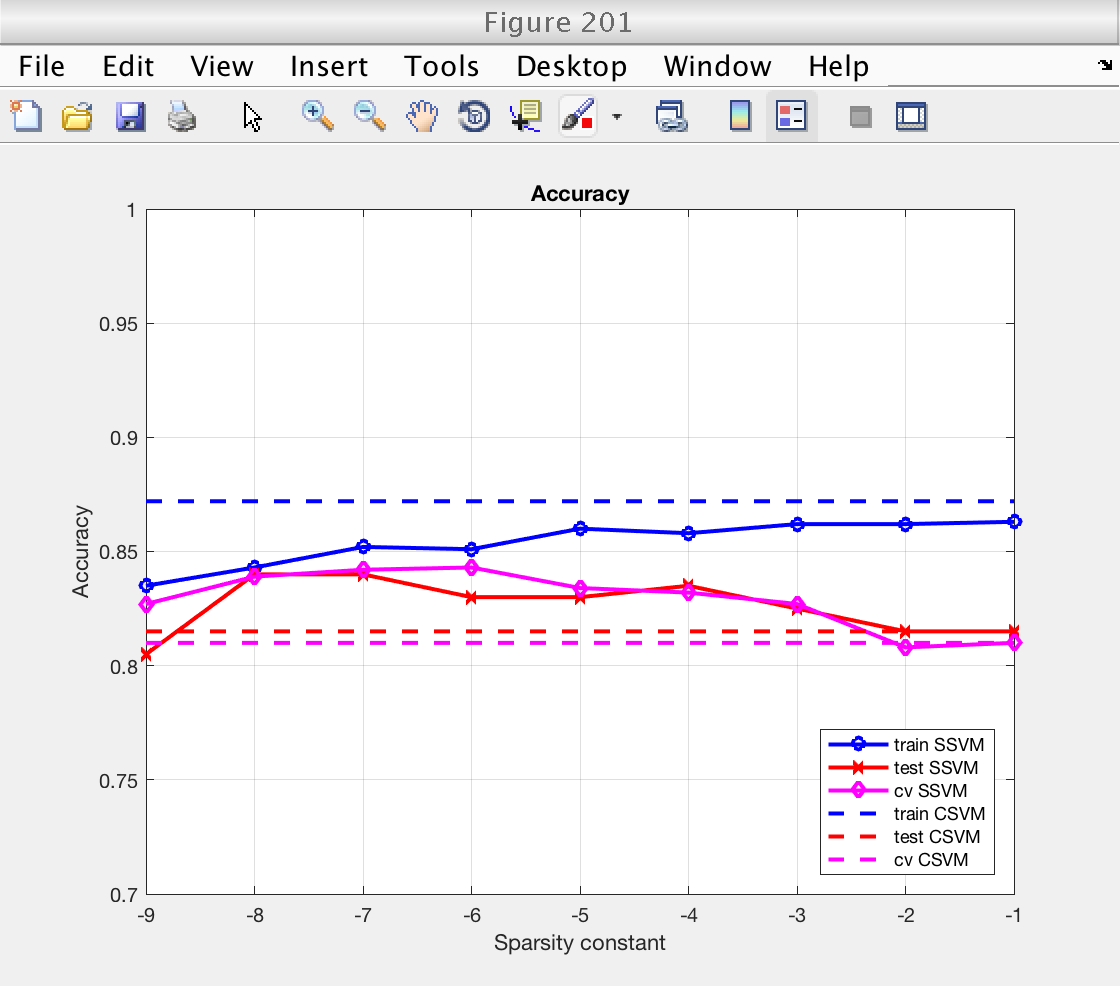
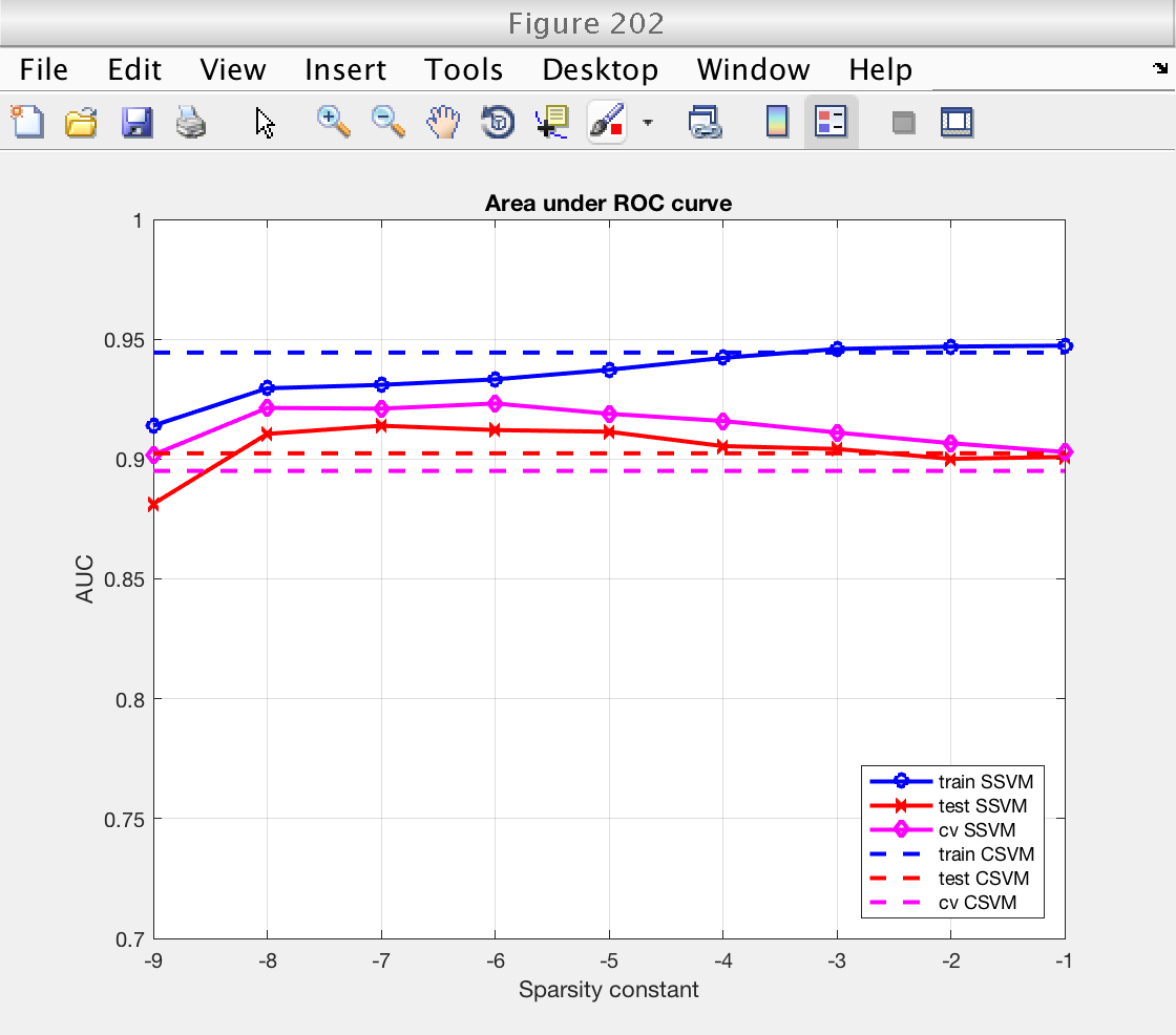
Figures: performance

Now we plot the classification performance. We compare training error, training error, and cross validation error.

For both performance measures (accuracy and AUC), we see that:

1) Performance measured on the training set is higher than on the testing set, as expected. The classifiers have already learned the training data, and performance measured using it is optimistic.

2) Performance measured by cross-validation lies between the two. It is an acceptable replacement for the testing error in situations where no testing data is available.

3) Performance (CV and testing set) for the sparse SSVM is larger than for the classical SVM for low sparsity levels. As we will see next, this is because the SSVM is only selecting a few important features and ignoring the redundant ones. In fact, for large values of the sparsity constant the SSVM starts using all features and the performance of both classifiers becomes similar (see next section).

% For classical SVM, repeat performance measures for all sparsity levels
nsp = length (ssvm_sp_vec);
acc_train_csvm = acc_train_csvm * ones (1, nsp);
acc_test_csvm  = acc_test_csvm * ones (1, nsp);
acc_cv_csvm    = acc_cv_csvm * ones (1, nsp);
auc_train_csvm = auc_train_csvm * ones (1, nsp);
auc_test_csvm  = auc_test_csvm * ones (1, nsp);
auc_cv_csvm    = auc_cv_csvm * ones (1, nsp);

log_sp = log2 (ssvm_sp_vec);

figure (201)
clf
plot (log_sp, acc_train_ssvm, 'bo-', 'LineWidth', 2)
hold on
plot (log_sp, acc_test_ssvm, 'rx-', 'LineWidth', 2)
plot (log_sp, acc_cv_ssvm, 'md-', 'LineWidth', 2)
plot (log_sp, acc_train_csvm, 'b--', 'LineWidth', 2)
hold on
plot (log_sp, acc_test_csvm, 'r--', 'LineWidth', 2)
plot (log_sp, acc_cv_csvm, 'm--', 'LineWidth', 2)
hold off
grid on
xlabel ('Sparsity constant')
ylabel ('Accuracy')
title ('Accuracy')
legend_text = {'train SSVM', 'test SSVM', 'cv SSVM', 'train CSVM', 'test CSVM', 'cv CSVM'};
legend (legend_text, 'Location', 'SouthEast')
ylim ([0.7 1])

figure (202)
clf
plot (log_sp, auc_train_ssvm, 'bo-', 'LineWidth', 2)
hold on
plot (log_sp, auc_test_ssvm, 'rx-', 'LineWidth', 2)
plot (log_sp, auc_cv_ssvm, 'md-', 'LineWidth', 2)
plot (log_sp, auc_train_csvm, 'b--', 'LineWidth', 2)
hold on
plot (log_sp, auc_test_csvm, 'r--', 'LineWidth', 2)
plot (log_sp, auc_cv_csvm, 'm--', 'LineWidth', 2)
hold off
grid on
xlabel ('Sparsity constant')
ylabel ('AUC')
title ('Area under ROC curve')
legend_text = {'train SSVM', 'test SSVM', 'cv SSVM', 'train CSVM', 'test CSVM', 'cv CSVM'};
legend (legend_text, 'Location', 'SouthEast')
ylim ([0.7 1])

Select optimal sparsity

We select the optimal sparsity level as the sparsest one that produces a performance level within 2% of maximum performance.

We will select it from AUC measured by cross-validation.

% Find the position of best accuracy
idx_sp_best = find (auc_cv_ssvm > max (auc_cv_ssvm) - 0.02, 1, 'first');

% Get best accuracy
sp_best = ssvm_sp_vec(idx_sp_best);

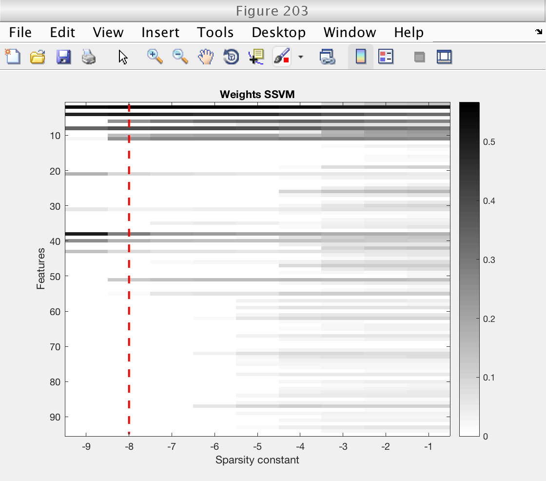
Figures: weights

First, we plot an image showing the weigts for the SSVM for each sparsity level. We indicate with a red dashed line the optimal sparsity level.

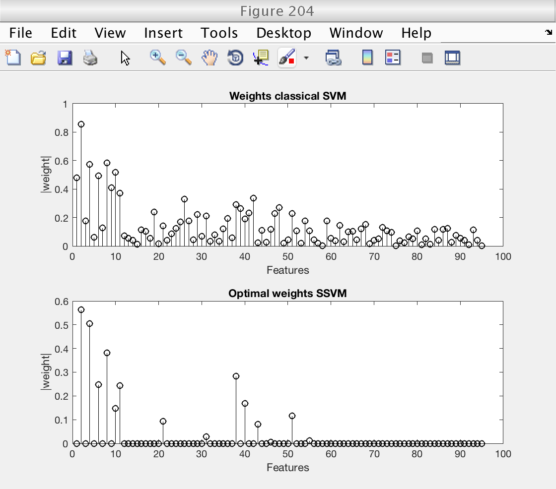
Then, we plot the weights selected by the classical SVM and compare them with the optimal weights selected by the SSVM.

Note that for low levels of sparsity, the SSVM essentially selects the original Ripley features (the first 10). Even more, only the second component of the Ripley features is selected, once for each copy (even features).

These plots clearly show that the improved performance of the SSVM comes from its ability of givin a zero weight to uninteresting features.

% Plot image of SSVM's weights, for each sparsity level
figure (203)
ymax = size (weights_ssvm, 2);
imagesc (log2 (ssvm_sp_vec), 1 : ymax, abs(weights_ssvm)')
hold on
plot (log2 (sp_best) * [1 1], [1 ymax], 'r--', 'LineWidth', 2)
hold off
colormap (1 - gray)
colorbar
xlabel ('Sparsity constant')
ylabel ('Features')
title ('Weights SSVM')

% Plot weights of classical SVM and optimal weights of SSVM
figure (204)
subplot (211)
stem (abs (weights_csvm), 'k')
xlabel ('Features')
ylabel ('|weight|')
title ('Weights classical SVM')
subplot (212)
stem (abs (weights_ssvm(idx_sp_best, :)), 'k')
xlabel ('Features')
ylabel ('|weight|')
title ('Optimal weights SSVM')

% Restore random stream
RandStream.setGlobalStream(s0);